But … why? Intuitively, one can probably see on a very high level why that might happen. However, what is the mathematical reason this happens, what is the proof that explains why this occurs? Let us explore this problem at a fundamental level and understand what the problem is and why it happens at its core.

Recurrent Neural Networks Fundamentals

We will begin with a brief but necessary review of what a recurrent neural network is and how we can formulate it formally.

A recurrent neural network is a neural network whose output will constitute part of its next input.

It’s important to note that the input depends both on the previous output and any new input the model might receive at any particular loop. Thus, RNNs function as neural networks that can “remember” information from past computations. The output of previous computations is simply propagated directly to newer states.

Take a look at a snapshot of the RNN flow at some timestamp $t$.

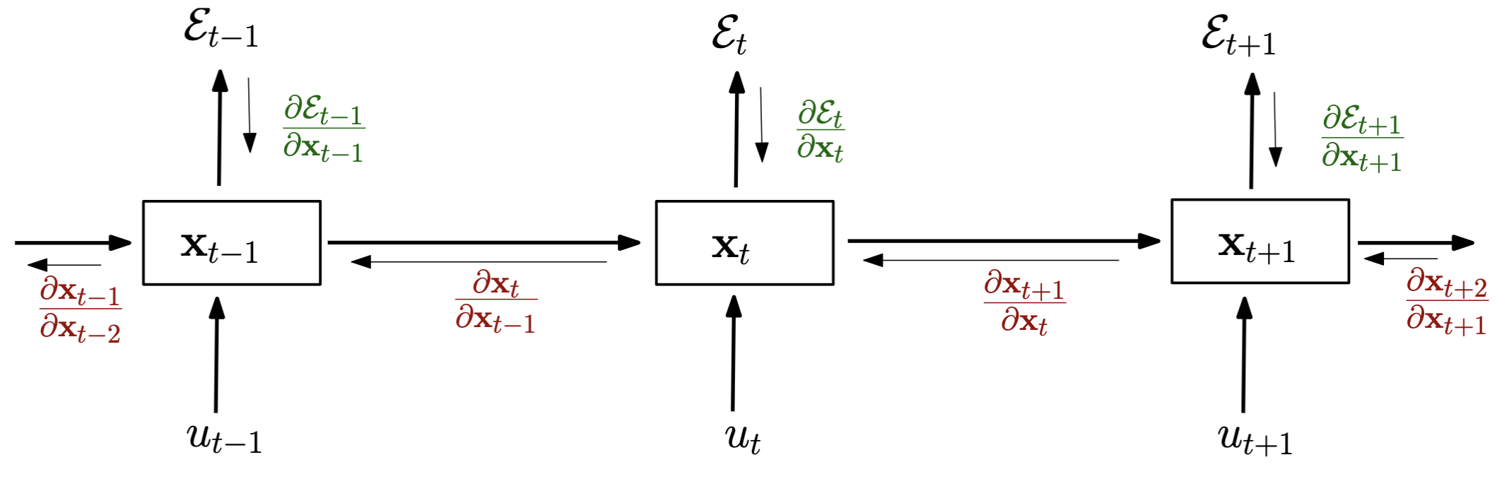
At each state we have a brand new input $u_t$, the previous output $x_{t-1}$ as additional input, output $x_t$, and a loss $\mathcal{E}_t$.

Unlike a traditional Neural Network, the loss is not simply defined on the final output since an RNN computes multiple outputs in a sequence. Each output produced demands a new loss computation $\mathcal{E}_t$

Why are we focusing on RNNs? They are a generalised version of multi-layered networks. They can have arbitrary depth due to their recursive nature making them ideal to demonstrate vanishing/exploding gradients.

Our findings will be applicable to any multi-layered network with the same foundational structure.

A Mathematical Formulation of RNN

Let us describe the RNN in algebraic terms. At each timestep $t$:

where $\theta$ are the model parameters - usually the weights $W$ of the model.

This formulation is intentionally broad and non-specific as to what the function $F$ actually looks like. In our case, for an RNN we will be looking at the following implementation:

where $W_{rec}$ (recurrent) are the weights that are multiplied with the previous output, $W_{in}$ is multiplied with the new input, $\sigma$ is an element-wise function (such as ReLU) to introduce non-linearity, and $b$ is the bias.

NOTE: This is one of the multiple potential implementations of an RNN. Here we only have one layer $W$ per timestep but we could have multiple. Also, $\sigma$ could be applied in a different way: $x_t = \sigma(W_{rec}x_{t-1} + W_{in} u_t + b)$.

We will stick with eq. (2) but note that implementation details can change, however the essence of the problem is the same. Eq. (2) is a “vanilla” implementation of RNN, and all findings can be applied to different implementations of RNN models.

Defining the Loss

With RNNs we are optimising for some type of error/loss. The specific loss function we utilize is arbitrary for this proof. For instance, it could be the difference of the output vector $x_t$ and some target $y_t$ squared (MSE). All we should care about is that our loss is a function of $x_t$, i.e. $\mathcal{E_t} = \mathcal{L}(x_t)$.

However, we can measure the loss of each output we produce at any timestep $t$. The question naturally arises: what is the final metric for which we are optimising for if we have multiple losses?

Here we could come up with all sorts of schemes. For instance, we could weigh the loss computations of the later stages higher than previous ones. To keep things simple, let us assume that we are simply considering all stages of the RNN to have an equal share of impact. We will assume that the final metric we are optimising for is the sum of all losses:

Optimising for the Loss

Now for the part we have building up to: let us optimise for the loss as defined above. We are trying to minimise the loss by altering the parameters of the model ($\theta$).

Remember, vanishing/exploding gradients affects our ability to optimise the loss. Here is where we start to show this.

Let us focus w.l.o.g. on some timestep $t$:

Let us pause here. We have two components.

First, $\frac{\partial\mathcal{E_t}}{\partial x_t}$ remains as is. The loss is a direct function of $x_t$. We cannot simplify further.

$\frac{\partial x_t}{\mathcal{\partial\theta}}$ is more involved. By looking at eq. (2) $x_t$ is a function of $W$ and $x_{t-1}$ (which is is also in turn implicitly a function of $W$). These are the two variables we care about since we are optimising for $\theta$ ($W$). $u_t$ and $b$ are irrelevant as they are not a function of $\theta$($W$).

Remember from multivariable calculus that if $x=g(t)$, $y=h(t)$, and $z = f(x, y)$, then $\frac{\partial z}{\partial t} = \frac{\partial z}{\partial x} \frac{\partial x}{\partial t} + \frac{\partial z}{\partial y} \frac{\partial y}{\partial t}$.

To make our case easier to read, let us make an auxiliary function $g(W) = W$. So:

Now it becomes easier to see that we can do the following:

which can be simplified to \(\begin{align} \boxed{\frac{\partial x_t}{\mathcal{\partial\theta}} = \frac{\partial x_t}{\mathcal{\partial g}} + \frac{\partial x_t}{\mathcal{\partial x_{t-1}}} \frac{\partial x_{t-1}}{\mathcal{\partial\theta}}} \end{align}\tag{7}\) Now we can expand: \(\begin{align} \Rightarrow \frac{\partial\mathcal{E_t}}{\mathcal{\partial\theta}} = \frac{\partial\mathcal{E_t}}{\partial x_t} \frac{\partial x_t}{\mathcal{\partial\theta}} &= \frac{\partial\mathcal{E_t}}{\partial x_t} [\frac{\partial x_t}{\mathcal{\partial g}} + \frac{\partial x_t}{\mathcal{\partial x_{t-1}}} \frac{\partial x_{t-1}}{\mathcal{\partial\theta}}]\\ &\boxed{= \frac{\partial\mathcal{E_t}}{\partial x_t}\frac{\partial x_t}{\mathcal{\partial g}} + \frac{\partial\mathcal{E_t}}{\partial x_t}\frac{\partial x_t}{\mathcal{\partial x_{t-1}}} \frac{\partial x_{t-1}}{\mathcal{\partial\theta}}}\\ \end{align}\tag{8.1}\)

Notice that the last term $\frac{\partial x_{t-1}}{\mathcal{\partial\theta}}$ can be recursively substituted using eq (7) which will result in an equation with $\frac{\partial x_{t-2}}{\mathcal{\partial\theta}}$ which will be recursively substituted, etc. till we reach $x_1$.

Thus, intuitively we should see the following pattern occurring in eq (8.1): \(\begin{align} \Rightarrow \frac{\partial\mathcal{E_t}}{\mathcal{\partial\theta}} &= \frac{\partial\mathcal{E_t}}{\partial x_t}\frac{\partial x_t}{\mathcal{\partial g}} + \frac{\partial\mathcal{E_t}}{\partial x_t}\boxed{\frac{\partial x_t}{\mathcal{\partial x_{t-1}}}} \frac{\partial x_{t-1}}{\mathcal{\partial\theta}}\\ &= \frac{\partial\mathcal{E_t}}{\partial x_t}\frac{\partial x_t}{\mathcal{\partial g}} + \frac{\partial\mathcal{E_t}}{\partial x_t}\boxed{\frac{\partial x_t}{\mathcal{\partial x_{t-1}}}} \frac{\partial x_{t-1}}{\partial g} +\frac{\partial\mathcal{E_t}}{\partial x_t}\boxed{\frac{\partial x_t}{\mathcal{\partial x_{t-1}}} \frac{\partial x_{t-1}}{\partial x_{t-2}}}\frac{\partial x_{t-2}}{\partial \theta}\\ &= \frac{\partial\mathcal{E_t}}{\partial x_t}\frac{\partial x_t}{\mathcal{\partial g}} + \frac{\partial\mathcal{E_t}}{\partial x_t}\boxed{\frac{\partial x_t}{\mathcal{\partial x_{t-1}}}} \frac{\partial x_{t-1}}{\partial g} + \frac{\partial\mathcal{E_t}}{\partial x_t}\boxed{\frac{\partial x_t}{\mathcal{\partial x_{t-1}}} \frac{\partial x_{t-1}}{\partial x_{t-2}}}\frac{\partial x_{t-2}}{\partial g} + \frac{\partial\mathcal{E_t}}{\partial x_t}\boxed{\frac{\partial x_t}{\mathcal{\partial x_{t-1}}} \frac{\partial x_{t-1}}{\partial x_{t-2}}\frac{\partial x_{t-2}}{\partial x_{t-3}}}\frac{\partial x_{t-3}}{\partial \theta}\\ &= ... \end{align}\tag{8.2}\)

The emerging structure is pretty clear and we can formulate it inefficiently as follows:

This can be simplified further. Notice that when taking the derivative of $x_t$ in terms of $x_k$ such that $k<t$ there is a linear and predictable relationship between each timestep.

That is, $x_t$ is a function of $x_{t-1}$ which is a function of $x_{t-2}$ which is a function of $x_{t-3}$ … until $x_k$. There are no other paths from $x_t$ to $x_k$. I.e. $x_t$ is not a function of both $x_{t-1}$ and $x_{t-2}$ or any other $x_j$ for some $j\neq t-1$.

Thus: \(\begin{align} \frac{\partial x_t}{\partial x_k} &= \frac{\partial x_t}{\partial x_{t-1}} \frac{\partial x_{t-1}}{\partial x_k}\\ &= \frac{\partial x_t}{\partial x_{t-1}} \frac{\partial x_{t-1}}{\partial x_{t-2}} \frac{\partial x_{t-2}}{\partial x_k}\\ &= ...\\ &= \prod_{j=k+1}^t \frac{\partial x_{j}}{\partial x_{j-1}} \end{align}\tag{10}\)

So, eq (9) gets further simplified to: \(\begin{align} \Rightarrow \frac{\partial\mathcal{E_t}}{\mathcal{\partial\theta}} &= \sum_{k=1}^t [\frac{\partial \mathcal{E}_t}{\partial x_t} \frac{\partial x_t}{\partial x_{k}}\frac{\partial x_k}{\partial g}] \end{align}\tag{11}\)

TL;DR, we derived a simple formula for optimising the loss at a timstep $t$.

Solving the Gradients

With the simplified formulation of what our loss looks like at timestep $t$, we will go a step further and start computing the gradients.

We will cheat here and focus directly on $\frac{\partial x_t}{\partial x_k}$. We already showed that $\frac{\partial x_t}{\partial x_k} = \prod_{j=k+1}^t \frac{\partial x_{j}}{\partial x_{j-1}}$.

So let us solve $\frac{\partial x_{j}}{\partial x_{j-1}}$:

Most resources skip this final calculation but we will go through step by step how to compute this to understand the derivation fully.

As a refresher, take a look at vector by vector partial derivatives. We will use numerator layout notation but it does not really matter in this case.

Let us denote $x_j^i$ as the $i$-th element of output vector $x$ at timestep $j$:

Going back to the beginning of this paragraph, we can now show the following: \(\begin{align} \frac{\partial x_t}{\partial x_k} = \prod_{j=k+1}^t \frac{\partial x_{j}}{\partial x_{j-1}} = \prod_{j=k+1}^t [W_{rec} diag(\sigma'(x_{j-1}))] \end{align}\tag{13}\)

This equation is crucial. We just showed that when optimising for the loss of an RNN we will inevitably have to deal with a gradient computation which involves multiplying $W_{rec}$ repeatedly with itself $t-k$ times. This intuitively means that the deeper the network the more times we will have to multiply with $W_{rec}$ and the more amplified the effect of the matrix will be. Let’s make this concrete.

Vanishing/Exploding the Gradients

“To understand this phenomenon we need to look at the form of each temporal component, and in particular at the matrix factors $\frac{\partial x_t}{\partial x_k}$ […] that take the form of a product of $t − k$ Jacobian matrices. In the same way a product of $t − k$ real numbers can shrink to zero or explode to infinity, so does this product of matrices (along some direction v)” (Pascanu et al).

A Linear Algebra Precursor

Before we step into the final part, let us introduce/recap a few concepts and formulas that will be important.

Singular values

A singular value of a matrix $\sigma(A)$ geometrically expresses the stretching factor in any direction. This is different than the eigenvalues of a matrix which only express the stretching factor along the direction of a matrix’s eigenvectors (which do not necessarily span the matrix’s space).

By extension, $\sigma_{max}(A)$ geometrically expresses the (absolute) maximum stretching factor in any direction.

Formally:

Spectral Norm (2-Norm) of a Matrix

The spectral norm of a matrix is just the max singular value:

Spectral Radius

The spectral radius of a matrix is a fancy term for the maximum (absolute) eigenvalue:

Spectral Norm + Spectral Radius

We are allowed to do this because all the eigenvalues of \(A^*A\) are non-negative. This is because \(A^*A\) is a Hermitian Positive Semi-Definite Matrix:

1. Hermitian: \((A^*A)^* = A^*A\)
2. PSD: \(x^* A^*A x = (Ax)^*(Ax) = \sum\limits_{i} {(Ax)_i ^2} \geq 0\)

Vanishing Gradients

Review equations (11) and (13). They have led us to this recursive multiplication of $W_{rec}$. Attempting to visualise how the vectors shrink and expand due to this product is difficult.

Instead we will focus on the “upper bound” of what this product produces: the (absolute) maximum stretching factor. The sign of the stretch does not matter. What matters is the magnitude of the stretch.

Consulting the Linear Algebra Precursor, we will go ahead and prove a sufficient condition for vanishing gradients:

Let us define an upper bound for $diag(\sigma’(x_{j-1}))$. Assume:

If \(\boxed{\sigma_{max}(W_{rec}) < \frac{1}{\gamma}}\), then long term components vanish (as $t \rightarrow \infty$):

Let us define an upper bound $\eta$:

Working our way upwards, let’s revisit eq. (11) and (13):

Since $\eta < 1$, as $t-k$ increases, the terms tend to go to 0. This means that events further in the past stop contributing to the future.

Thus, under the requirement that $\sigma_{max}(W_{rec}) < \frac{1}{\gamma}$, the model becomes unable to consider events in the past and bases its predictions on recent events. The vanishing gradients make the model “forget” past events easily (ie. past events do not contribute to future outcomes).

Exploding Gradients

Just as gradients can vanish due to the repeated multiplication of $W_{rec}$, they can similary “explode”. We will skip the full proof as it is almost identical to the vanishing gradients one we showed above.

However, notice how we used the following inequality to formulate our proof above:

The direction of the inequality prohibits us for using it to prove the inverse of the vanishing gradients. Thus, we cannot form a sufficient condition but only a necessary one:

For the exploding gradients problem to appear we need: \(\boxed{\sigma_{max}(W_{rec}) > \frac{1}{\gamma}}\), with \(\|diag(\sigma'(x_{j-1}))\|_2 > \gamma\). Long term components will then be able to explode (as $t \rightarrow \infty$).

Notes

This article was heavily based on the paper by Pascanu et al. which explores the problem of vanishing gradients at great technical detail.

I tried keeping the notation on par with their paper as well as other sources to maintain consistency.

On a minor note, the paper on equation (5) has a minor algebraic error on $W^T_{rec}diag(\sigma’(x_{i-1}))$. Tracing the equation that leads to this result (as we showed in this article) actually leads to $W_{rec}diag(\sigma’(x_{i-1}))$. Even if we decide to not use numerator layout notation, the outcome is still different. However, this does not cause any fundamental error in the findings of their paper.

References

• Pascanu, R., Mikolov, T., & Bengio, Y. (2012). On the difficulty of training Recurrent Neural Networks. arXiv. https://doi.org/10.48550/arxiv.1211.5063
• “Matrix Norm.” Wikipedia, Wikimedia Foundation, 25 Apr. 2026, Matrix_norm
• “Vanishing Gradient Problem.” Wikipedia, Wikimedia Foundation, 30 Sept. 2025, Vanishing_gradient_problem.